Model objects and predicting whole brain activity
Model objects are supereeg’s class that contains the correlation model that we use to reconstruct full-brain activity from recordings at an impoverished set of locations. The supereeg package offers a several pre-compiled models that you can use to reconstruct brain activity. We also provide several ways of creating or specifying your own model. This tutorial will review how to use the pre-made models included in this package and make a new model from scratch.
Load in the required libraries
import warnings
warnings.simplefilter("ignore")
%matplotlib inline
import supereeg as se
import numpy as np
First, let’s load in our default model, example_model, that we made
from the pyFR
dataset
resampled to 20mm cubic voxels.
model = se.load('example_model')
other model options: - pyFR_k10r20_6mm: correlation model trained on
the pyFR dataset and resampled to 6mm cubic voxels
pyFR_k10r20_20mm: full name ofexample_model(either string will load the same model)
Initialize model objects
Model objects can be initialized by passing any of the following to the
Model class instance initializer: - a path to an existing saved
model object (ending in .mo) - an existing model object (this makes
a copy of the existing model object) - a Brain object or Nifti
object [or paths to saved Brain objects (.bo) or Nifti objects
(.nii)] - a string corresponding to any of the built-in example
files,
of any format (any datatype may be converted to a Model object)
In addition, new model objects may be created via the load function
(which loads any of the toolbox-supported data types) and specifying
return_type='mo'
nii_mo = se.Model('example_nifti')
Or:
nii_mo = se.load('example_nifti', return_type='mo')
Model object methods
There are a few other useful methods on a model object:
mo.info()
This method will give you a summary of the model object:
model.info()
Number of locations: 210
Number of subjects: 67
RBF width: 20
Date created: Fri Jul 27 16:19:31 2018
Meta data: {'stable': True}
mo.plot_data()
This method will plot your model.
The model is comprised of a number of fields. The most important are the
model.numerator and model.denominator. Dividing these two fields
gives a matrix of z-values, where the value in each cell represents the
covariance between every model brain location with every other model
brain location. To view the model, simply call the model.plot
method. This method wraps seaborn.heatmap to plot the model
(transformed from z to r), so any arguments that seaborn.heatmap
accepts are supported by model.plot.
model.plot_data(xticklabels=False, yticklabels=False)
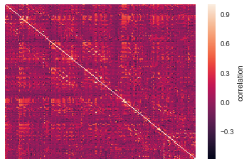
<matplotlib.axes._subplots.AxesSubplot at 0x117f13d10>
mo.update()
This method allows you to update the model with addition subject data.
To do this, we can use the update method, passing a new subjects
data as a brain object. First, let’s load in an example subjects data:
bo = se.load('example_data')
bo.info()
Number of electrodes: 64
Recording time in seconds: [ 5.3984375 14.1328125]
Sample Rate in Hz: [256, 256]
Number of sessions: 2
Date created: Fri Mar  9 17:09:35 2018
Meta data: {'patient': u'CH003'}
Now you can update the model with that brain object. This can be done
either in place using inplace = True, or you can save a new updated
model:
updated_model = model.update(bo, inplace=False)
updated_model.info()
Number of locations: 274
Number of subjects: 68
RBF width: 20
Date created: Fri Jul 27 16:19:31 2018
Meta data: {'stable': True}
You can also update the model by adding two model objects together.
mo_bo = se.Model(bo, locs=updated_model.get_locs(), n_subs=1)
mo_mo = se.Model(model, locs=updated_model.get_locs(), n_subs=67)
added_model = mo_mo + mo_bo
np.allclose(added_model.get_model(), updated_model.get_model())
True
You can subtract models too, but once this operation is performed, you won’t be able to update the model in the future.
new_locs = se.simulate_locations(n_elecs=100)
mo_bo = se.Model(bo, locs=new_locs, n_subs=1)
add_model = mo_bo + mo_bo
sub_model = add_model - mo_bo
np.allclose(mo_bo.get_model(), sub_model.get_model())
True
try:
    assert sub_model + add_model
except AssertionError:
    assert True == True
Note that the model is now comprised of 67 subjects, instead of 66 before we updated it.
mo.get_model()
This method returns the model in the form of a correlation matrix.
updated_model.get_model()
array([[ 1.        , -0.09811393,  0.18961899, ...,  0.27256808,
         0.36030263,  0.25768555],
       [-0.09811393,  1.        ,  0.23203525, ...,  0.37158962,
         0.07614721, -0.01200328],
       [ 0.18961899,  0.23203525,  1.        , ...,  0.01061833,
        -0.02072749,  0.1670675 ],
       ...,
       [ 0.27256808,  0.37158962,  0.01061833, ...,  1.        ,
         0.08097902,  0.15267173],
       [ 0.36030263,  0.07614721, -0.02072749, ...,  0.08097902,
         1.        , -0.03895988],
       [ 0.25768555, -0.01200328,  0.1670675 , ...,  0.15267173,
        -0.03895988,  1.        ]])
mo.save(fname='something')
This method will save the brain object to the specified file location.
The data will be saved as a ‘bo’ file, which is a dictionary containing
the elements of a brain object saved in the hd5 format using
deepdish.
#mo.save(fname='model_object')
Creating a new model
In addition to including a few pre-made models in the supereeg
package, we also provide a way to construct a model from scratch.
Created from a list of brain objects:
For example, if you have an ECoG dataset, we provide a way to construct a model that will predict whole brain activity. The more subjects you include in the model, the better it will be! To create a model, first you’ll need to format your subject data into brain objects. For the purpose of demonstration, and to highlight the “simulation” features of the toolbox, we will generate a synthetic ECoG dataset. Specifically, we’ll simulate data from 100 locations from each of 10 subjects and construct the model from that data:
# simulate 100 locations
locs = se.simulate_locations(100)

# simulate 10 brain objects to create a model
n_subs = 10
model_bos = [se.simulate_model_bos(n_samples=1000, sample_rate=1000, sample_locs=20,
                                   locs=locs, cov='toeplitz') for x in range(n_subs)]

model_bos[0].info()
Number of electrodes: 20
Recording time in seconds: [1.]
Sample Rate in Hz: [1000]
Number of sessions: 1
Date created: Fri Jul 27 16:20:32 2018
Meta data: {}
As you can see above, each simulated subject has 10 (randomly placed)
‘electrodes,’ with 1 second of data each. To construct a model from
these brain objects, simply pass them to the se.Model class, and a
new model will be generated:
new_model = se.Model(data=model_bos, locs=locs)
new_model.info()
Number of locations: 100
Number of subjects: 1
RBF width: 20
Date created: Fri Jul 27 16:20:32 2018
Meta data: {'stable': True}
Created by adding to model object fields:
Another option is to add a model directly.
You can add your model to model.data and add the corresponding
locations for the model in the field locs.
Another option, allows you to add your model to model.numerator,
which comprises the sum of the z-scored correlation matrices over
subjects. The model.denominator field comprises the sum of the
number of subjects contributing to each matrix cell in the
model.numerator field. You can add the locations for the model in
the field locs and the number of subjects to n_subs.
In this next example, we’re constructing the model from a toeplitz
matrix with 10 subjects using 100 simulated locations. We created the
matrix using the function, se.create_cov and added it to the
model.data field.
You can also create a custom covariance matrix in se.create_cov by
simply passing numpy array as and that is number of locations by number
of locations to cov and the number of location to n_elecs.
R = se.create_cov(cov='toeplitz', n_elecs=len(locs))
p = 10
toe_model = se.Model(data=R, locs=locs, n_subs=p)
toe_model.plot_data(xticklabels=False, yticklabels=False)
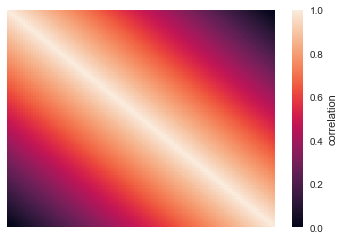
<matplotlib.axes._subplots.AxesSubplot at 0x118ce4750>
In this example we simulated 100 MNI locations. However coordinates can
also be derived by specifiying a template nifti file.
# new_model = se.Model(bos, template='/your/custom/MNI_template.nii')
Predicting whole brain activity
mo.predict()
Now for the magic. supereeg uses *gaussian process regression*
to infer whole brain activity given a smaller sampling of electrode
recordings. To predict activity, simply call the predict method of a
model and pass the subjects brain activity that you’d like to
reconstruct:
mo.predict(nearest_neighbor=True)
As default, the nearest voxel for each subject’s electrode location is
found and used as revised electrodes location matrix in the prediction.
If nearest_neighbor is set to False, the original locations are
used in the prediction.
mo.predict(force_update=False)
As default, the model is not updated with the subject’s correlation
matrix. By setting force_update to True, you will update the
model with the subject’s correlation matrix.
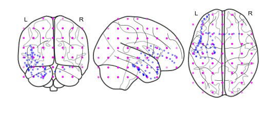
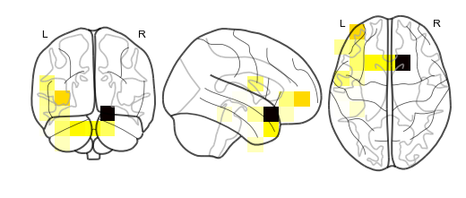
# plot a slice of the original data
print('BEFORE')
print('------')
bo.info()
nii = bo.to_nii(template='gray', vox_size=20)
nii.plot_glass_brain()
# voodoo magic
bor = model.predict(bo, nearest_neighbor=False, force_update=True)
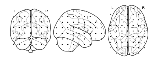
# plot a slice of the whole brain data
print('AFTER')
print('------')
bor.info()
nii = bor.to_nii(template='gray', vox_size=20)
nii.plot_glass_brain()
BEFORE
------
Number of electrodes: 64
Recording time in seconds: [ 5.3984375 14.1328125]
Sample Rate in Hz: [256, 256]
Number of sessions: 2
Date created: Fri Mar  9 17:09:35 2018
Meta data: {'patient': u'CH003'}
AFTER
------
Number of electrodes: 274
Recording time in seconds: [ 5.3984375 14.1328125]
Sample Rate in Hz: [256, 256]
Number of sessions: 2
Date created: Fri Jul 27 16:21:12 2018
Meta data: {}
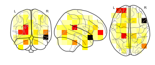
Using the supereeg algorithm, we’ve ‘reconstructed’ whole brain
activity from a smaller sample of electrodes.
You can plot locations of the new brain object with predicted activity. Observed locations are in black and predicted locations are in red.
bor.plot_locs()